scale_duke_discrete()

This vignette is intended to demonstrate the functionality of scale_duke_discrete(). The function allows users to utilize a discrete color scale of Duke official branding colors on ggplot2 visualizations. It is fully integrated with ggplot2 visualizations.

Plot Examples

For these visualization, we will use the R dummy data set palmerpenguins.

#install.packages("palmerpenguins")
library(palmerpenguins)
library(duke)
library(ggplot2)
library(ggmosaic)
attach(penguins)

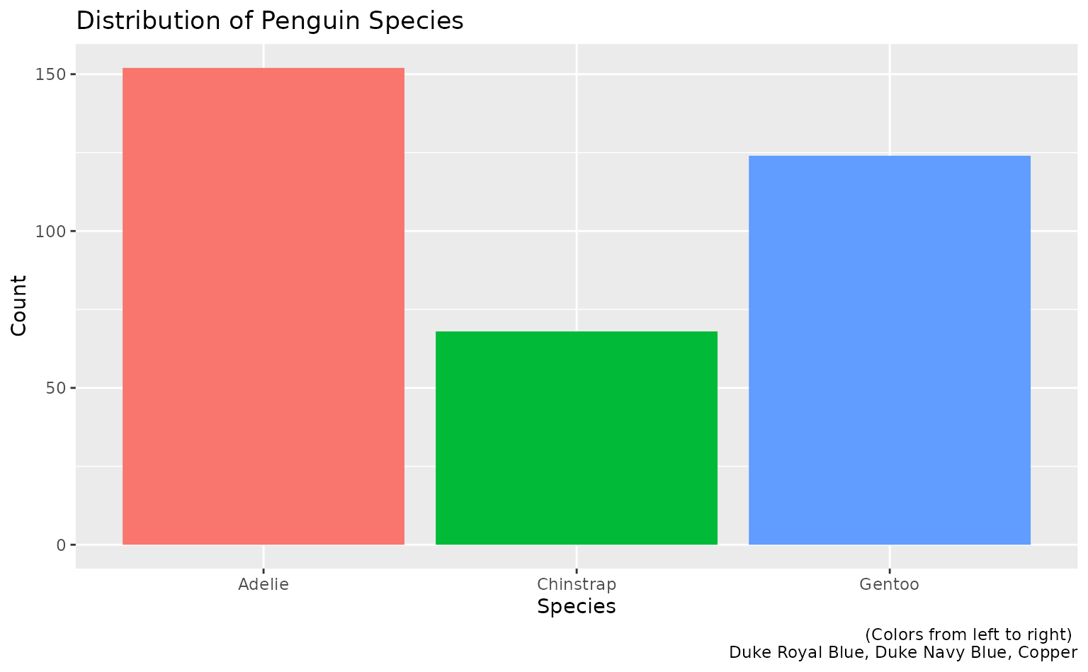
Bar Plot

plot <- ggplot(palmerpenguins::penguins, aes(x=species, fill = species)) +
  geom_bar() +
  labs(title = "Distribution of Penguin Species", caption = "(Colors from left to right) \n Duke Royal Blue, Duke Navy Blue, Copper", x = "Species", y = "Count") +
  theme(legend.position = "none")

plot +
  scale_duke_discrete()

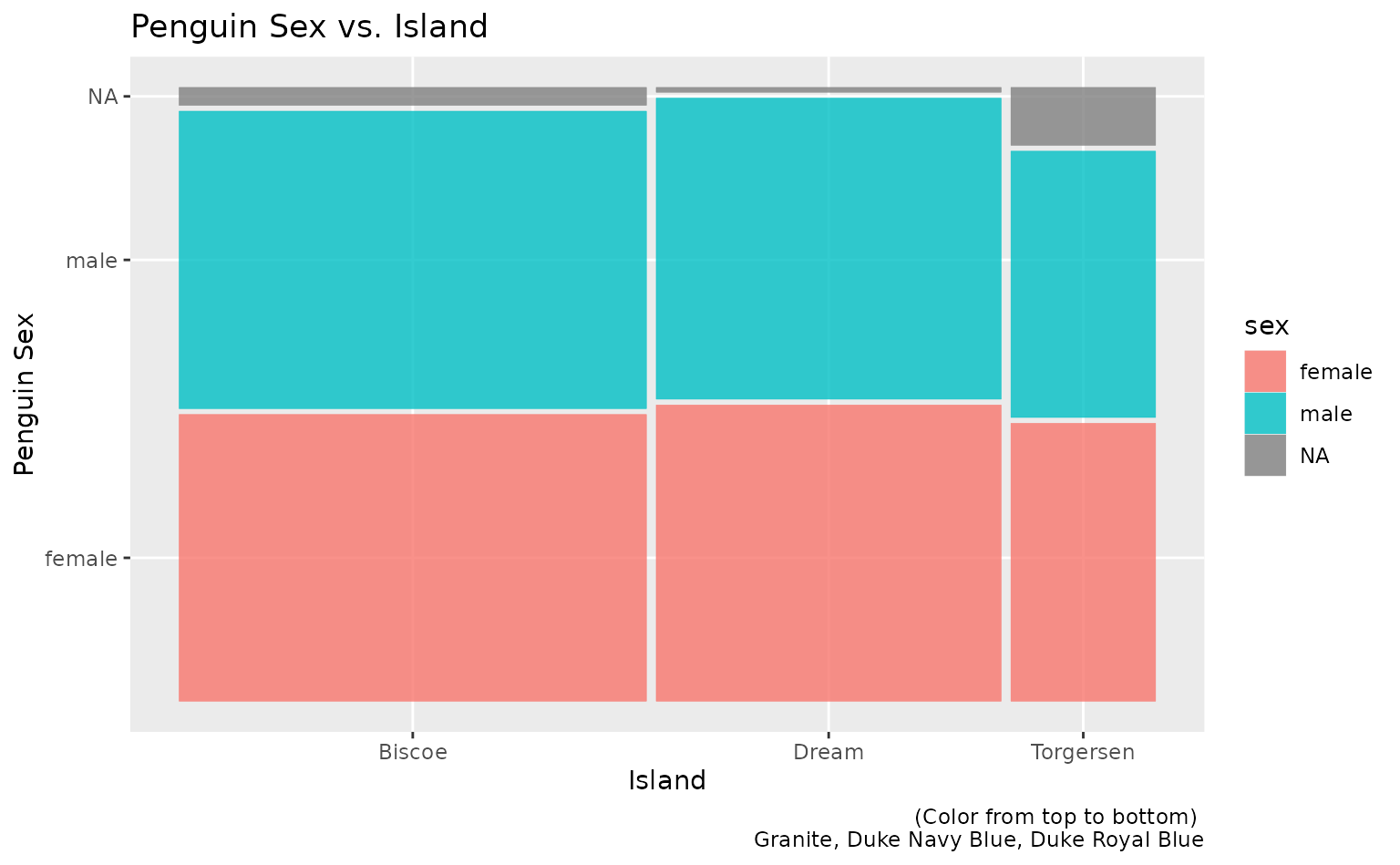
Mosaic Plot

plot2 <- ggplot(data = palmerpenguins::penguins) +
  ggmosaic::geom_mosaic(aes(x=product(sex, island), fill = sex)) +
  labs(title = "Penguin Sex vs. Island", x = "Island", y = "Penguin Sex", caption = "(Color from top to bottom) \n Granite, Duke Navy Blue, Duke Royal Blue")

plot2 +
  scale_duke_discrete()
#> Warning: `unite_()` was deprecated in tidyr 1.2.0.
#> ℹ Please use `unite()` instead.
#> ℹ The deprecated feature was likely used in the ggmosaic package.
#>   Please report the issue at <https://github.com/haleyjeppson/ggmosaic>.

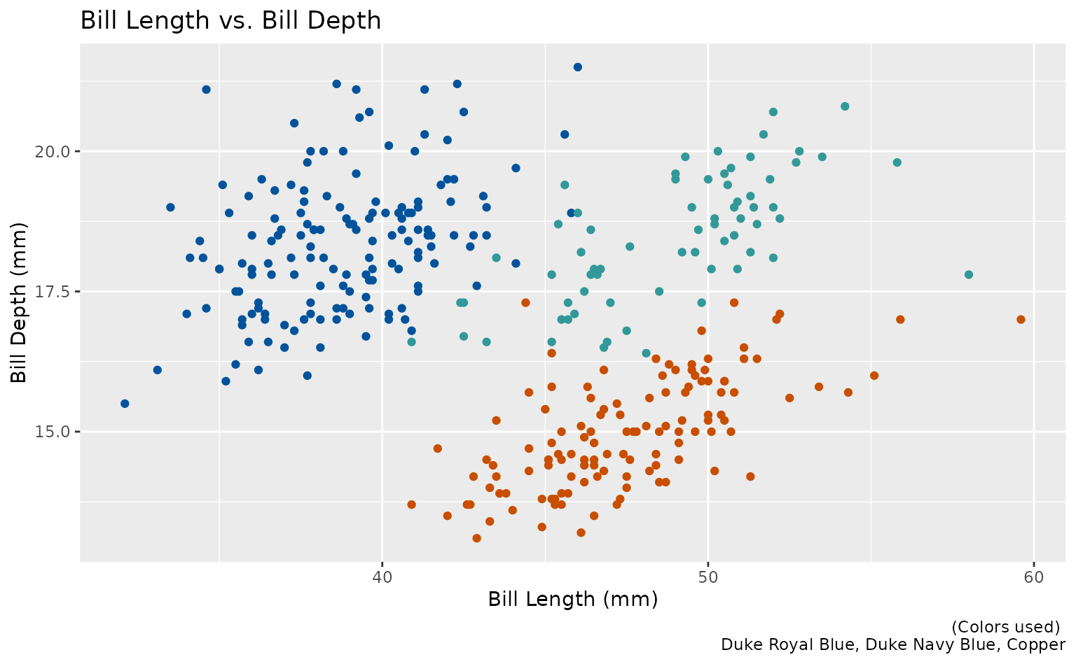
## Scatter Plot

plot3 <- ggplot(palmerpenguins::penguins, aes(x=bill_length_mm, y = bill_depth_mm)) +
  geom_point(aes(color = species)) +
  labs(title = "Bill Length vs. Bill Depth", caption = "(Colors used) \n Duke Royal Blue, Duke Navy Blue, Copper", x = "Bill Length (mm)", y = "Bill Depth (mm)")

plot3 + 
  scale_duke_discrete()
#> Warning: Removed 2 rows containing missing values (`geom_point()`).
#> New names:
#> • `colour` -> `colour...1`
#> • `colour` -> `colour...3`

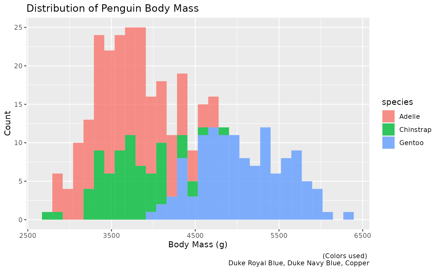
## Using scale_duke_discrete() on histogram plots

plot4 <- ggplot2::ggplot(palmerpenguins::penguins, aes(body_mass_g)) +
  geom_histogram(ggplot2::aes(fill = species), alpha = 0.8) +
  labs(title = "Distribution of Penguin Body Mass", caption = "(Colors used) \n Duke Royal Blue, Duke Navy Blue, Copper", x = "Body Mass (g)", y = "Count")

plot4 + scale_duke_discrete()
#> `stat_bin()` using `bins = 30`. Pick better value with `binwidth`.
#> Warning: Removed 2 rows containing non-finite values (`stat_bin()`).