library(duke)
library(palmerpenguins)
library(dplyr)
#>
#> Attaching package: 'dplyr'
#> The following objects are masked from 'package:stats':
#>
#>     filter, lag
#> The following objects are masked from 'package:base':
#>
#>     intersect, setdiff, setequal, union
library(ggplot2)
library(ggmosaic)
This vignette aims to comprehensively demonstrate the use and
functionality of the package duke. duke is
fully integrated with the ggplot2 and allows for the
creation of Duke official branded visualizations that are color blind
friendly.
student_names <- c("Jack", "Annie", "Paul", "Aidan", "Jake", "Josh", "Grace", "Suzy", "Beth", "Taylor", "Tanner", "Lisa", "Jimmy", "Larry", "Patricia", "Laura", "Yasmin", "Tim")
student_grades <- c("A+", "B", "A+", "C", "D", "A+", "E", "C", "B-", "B-", "D", "A-", "B+", "A-", "A-", "D", "B", "E")

students <- tibble(student = student_names, grade = student_grades)
Scatter Plot - Continuous Color
plot <- ggplot(penguins, aes(x = bill_length_mm, y = bill_depth_mm)) +
  geom_point(aes(color = body_mass_g)) +
  labs(
    title = "Bill Length vs. Bill Depth",
    x = "Bill Length (mm)",
    y = "Bill Depth (mm)"
  )

plot +
  scale_duke_continuous() +
  theme_duke()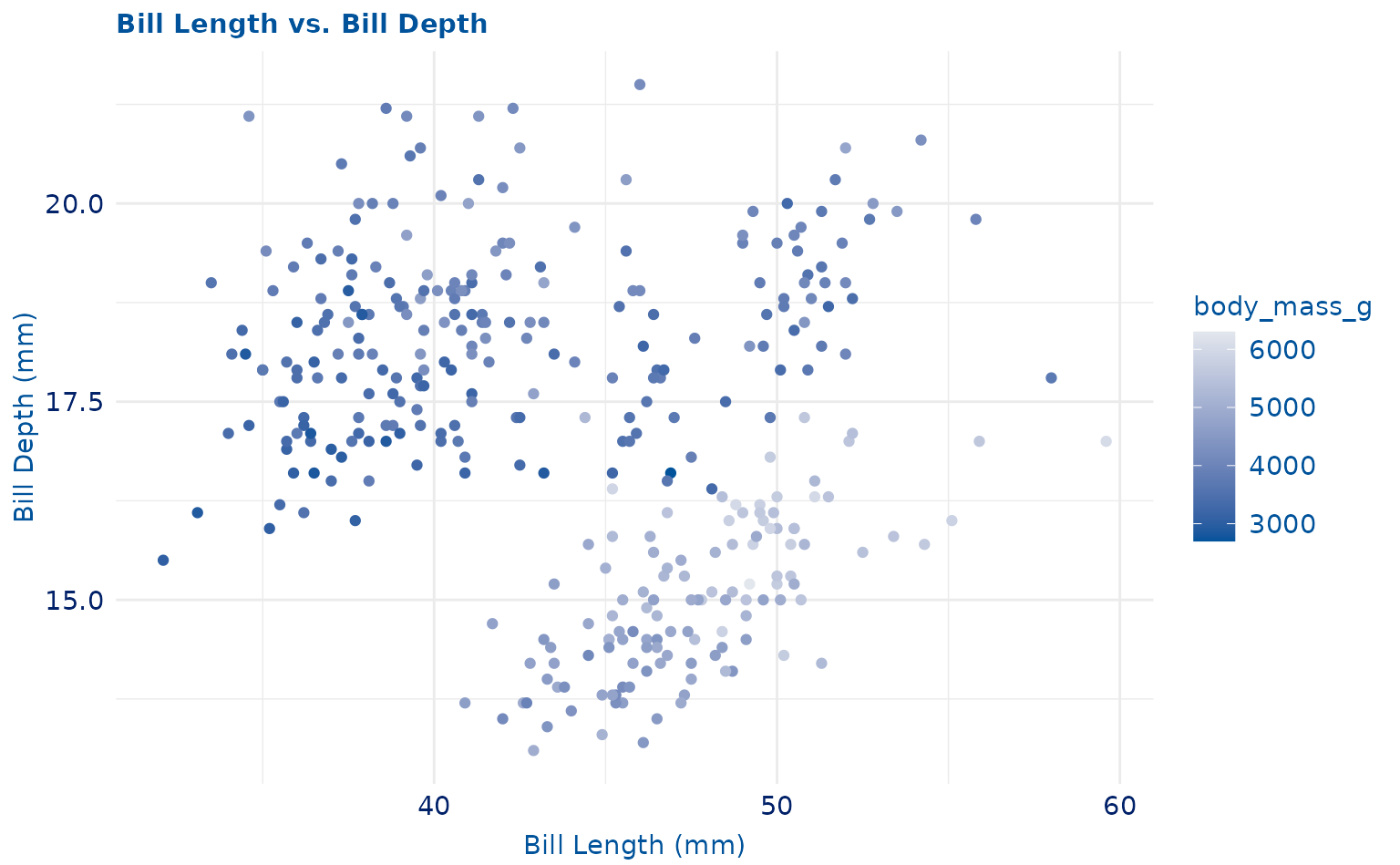
plot +
  geom_point(aes(shape = species)) +
  scale_duke_continuous() +
  theme_duke()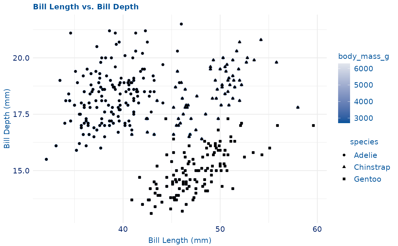
plot +
  scale_duke_continuous() +
  theme_minimal()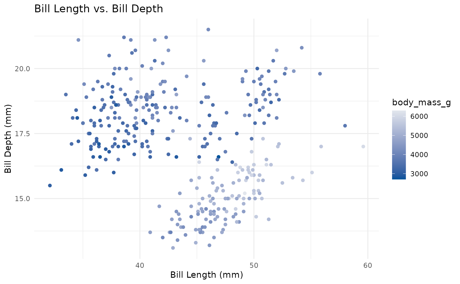
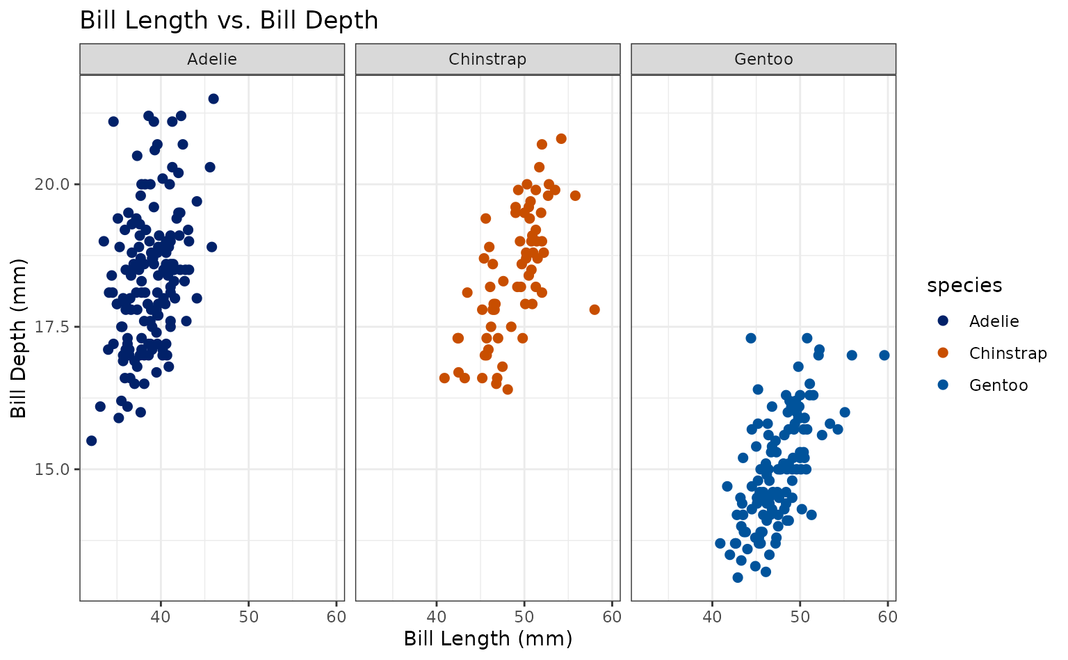
Scatter Plot - Discrete Color
plot1 <- ggplot(penguins, aes(x = bill_length_mm, y = bill_depth_mm, color = species)) +
  geom_point(size = 2) +
  labs(title = "Bill Length vs. Bill Depth", x = "Bill Length (mm)", y = "Bill Depth (mm)")

ggplot(penguins, aes(x = bill_length_mm, y = bill_depth_mm)) +
  geom_point(aes(color = species)) +
  labs(
    title = "Bill Length vs. Bill Depth",
    subtitle = "This is the subtitle",
    caption = "All text is in Duke Royal Blue",
    x = "Bill Length (mm)",
    y = "Bill Depth (mm)"
  ) +
  facet_wrap(~species) +
  theme_duke() +
  scale_duke_color_discrete()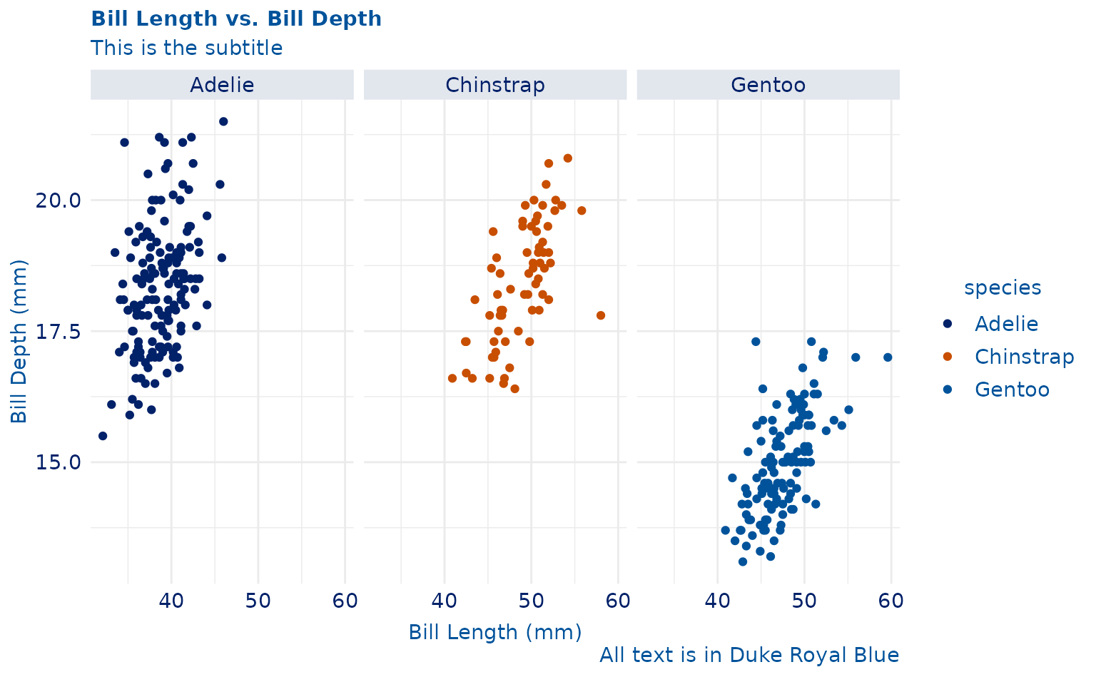
plot1 +
  theme_duke() +
  scale_duke_color_discrete()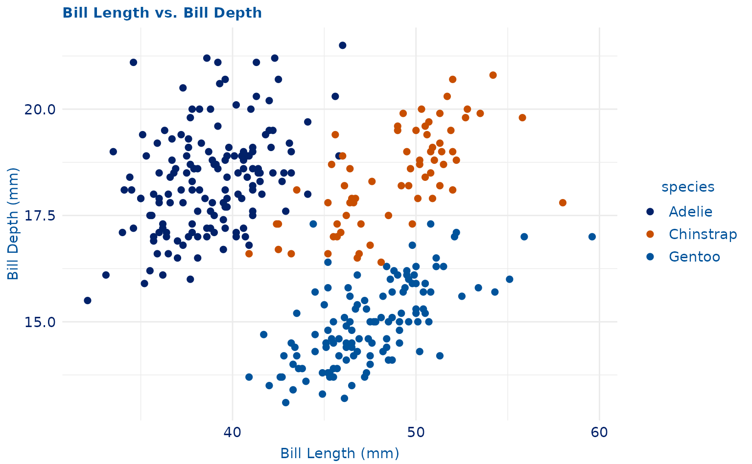
plot1 +
  scale_duke_color_discrete() +
  theme_minimal()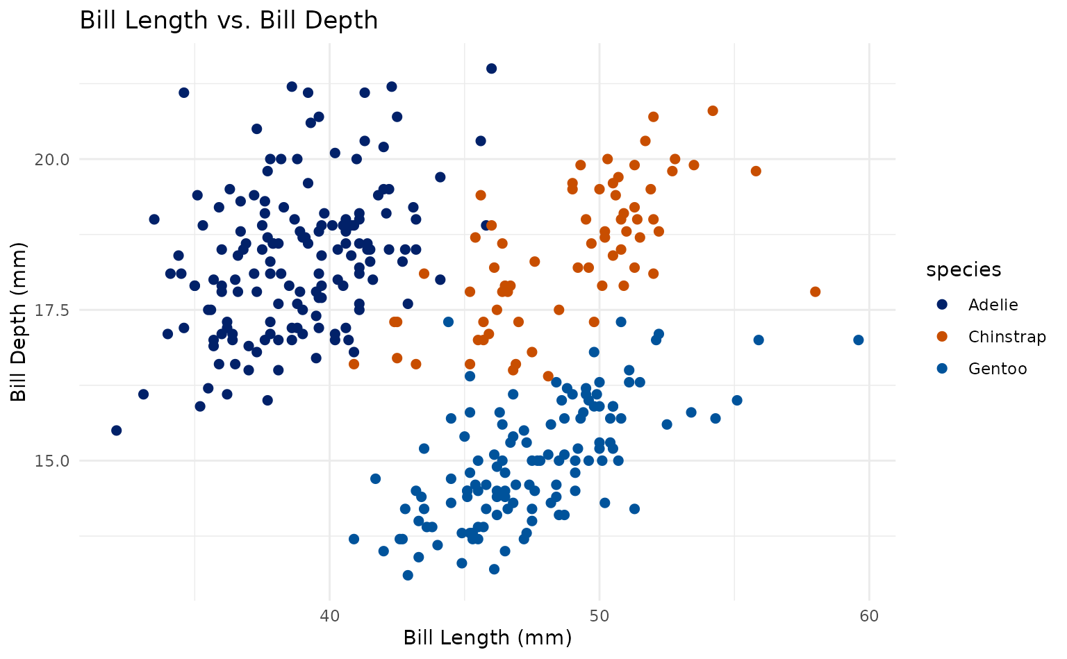
Bar Plot
plot2 <- ggplot(penguins, aes(x = species, fill = species)) +
  geom_bar() +
  labs(title = "Distribution of Penguin Species", x = "Species", y = "Count")

m_penguins <- penguins %>%
  dplyr::filter(sex == "male")

plot2.1 <- ggplot(m_penguins, aes(x = sex, fill = sex)) +
  geom_bar()

plot2.1 +
  scale_duke_fill_discrete() +
  theme_duke()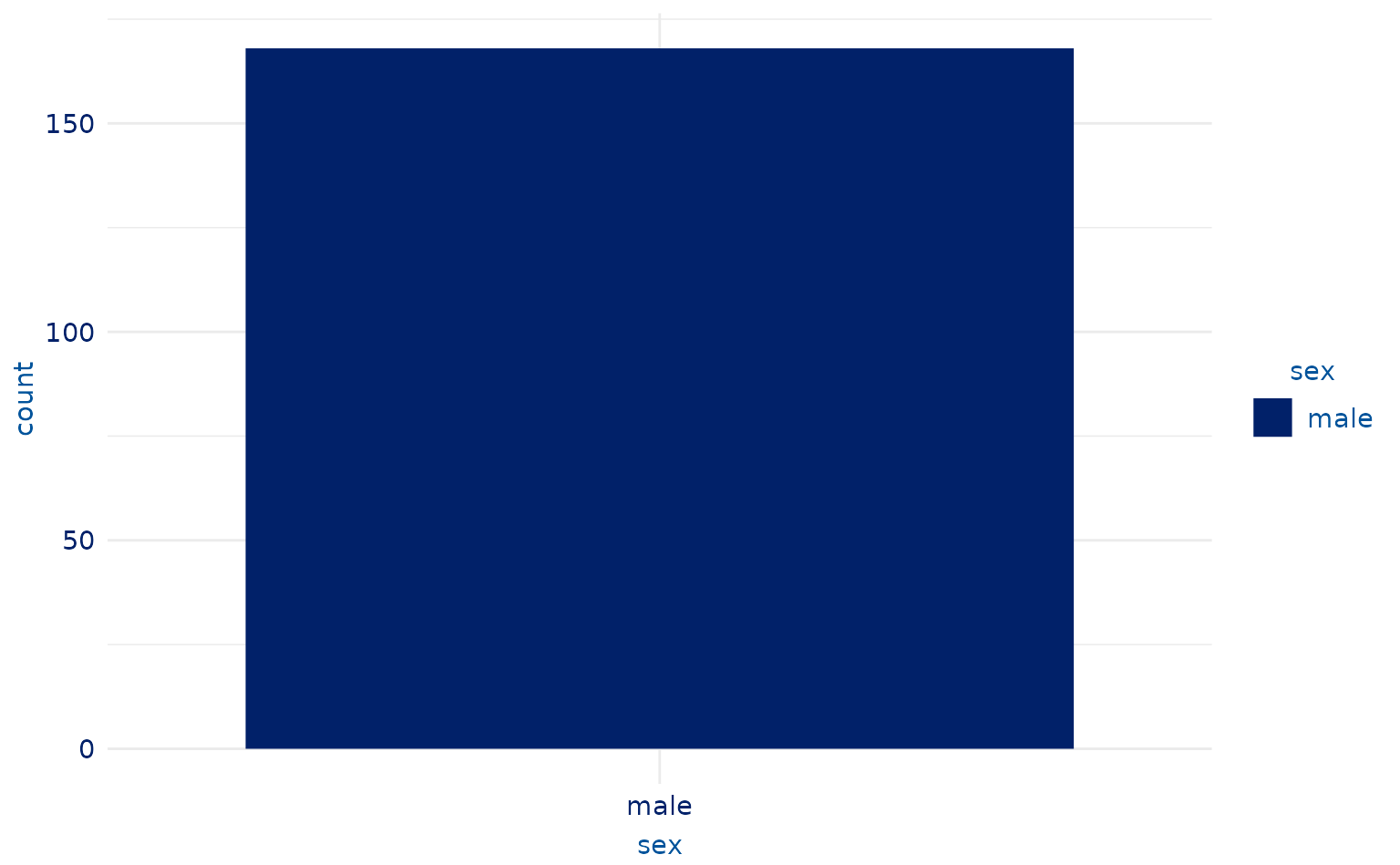
# 8-category plot
plot2.2 <- ggplot(students, aes(x = grade, fill = grade)) +
  geom_bar()

plot2.2 +
  scale_duke_fill_discrete() +
  theme_duke()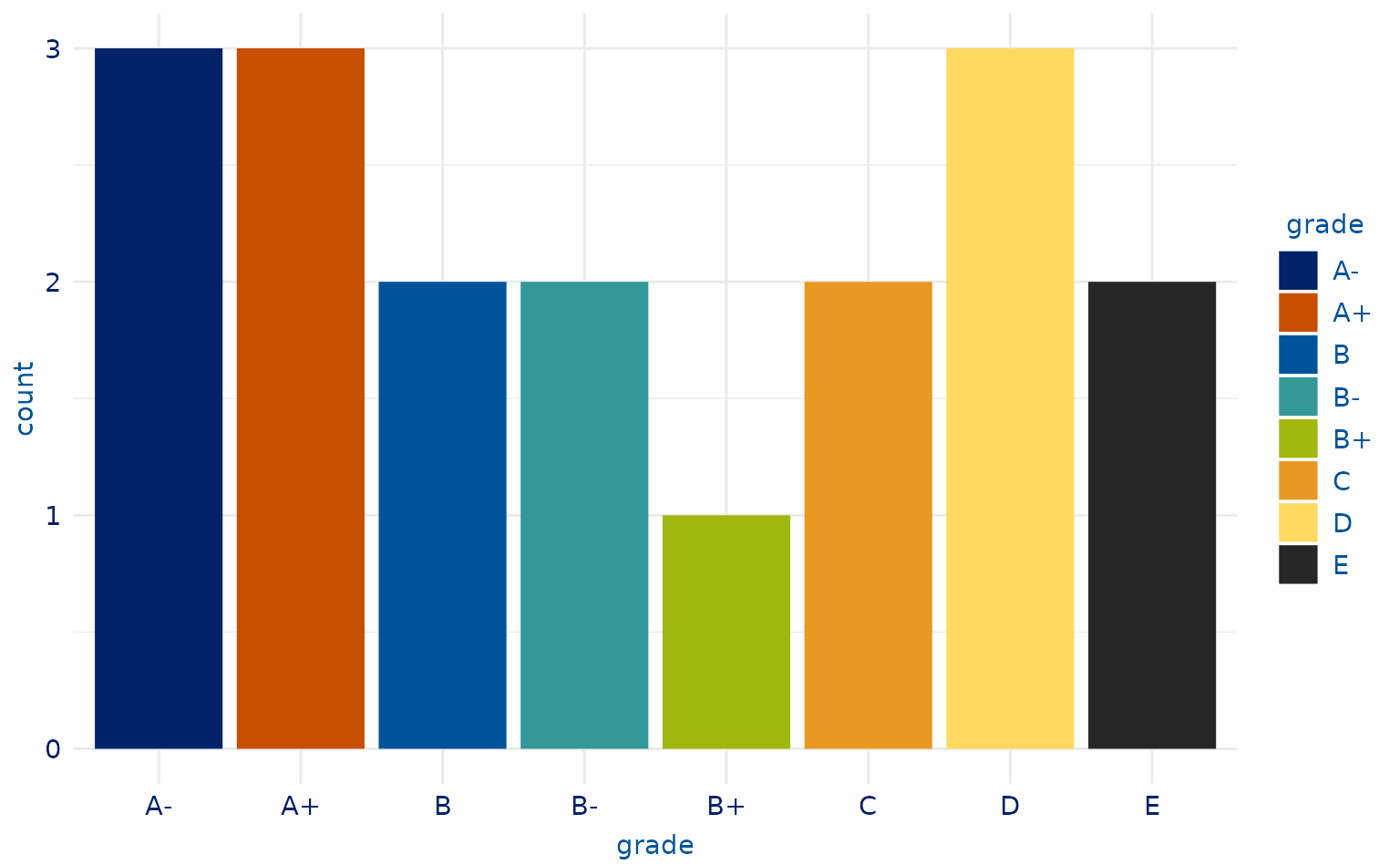
# 7-category plot
plot2.3 <- students %>%
  slice(-13) %>%
  ggplot(aes(x = grade, fill = grade)) +
  geom_bar()

plot2.3 +
  scale_duke_fill_discrete() +
  theme_duke()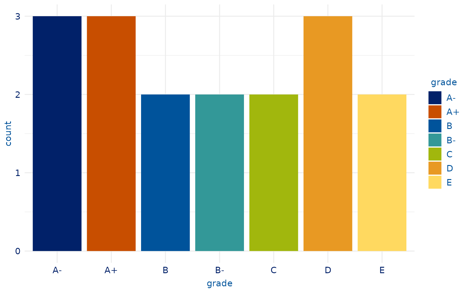
# 6-category plot
plot2.4 <- students %>%
  slice(-c(9, 10, 13)) %>%
  ggplot(aes(x = grade, fill = grade)) +
  geom_bar()

plot2.4 +
  scale_duke_fill_discrete() +
  theme_duke()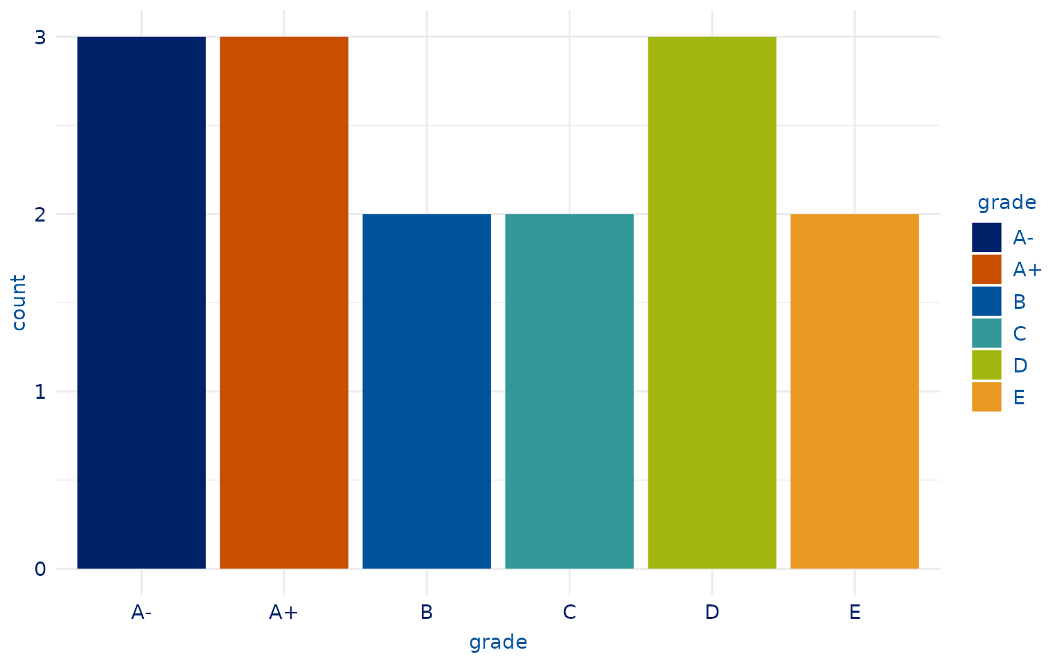
# 5-category plot
plot2.4 <- students %>%
  slice(-c(9, 10, 13, 7, 18)) %>%
  ggplot(aes(x = grade, fill = grade)) +
  geom_bar()

plot2.4 +
  scale_duke_fill_discrete() +
  theme_duke()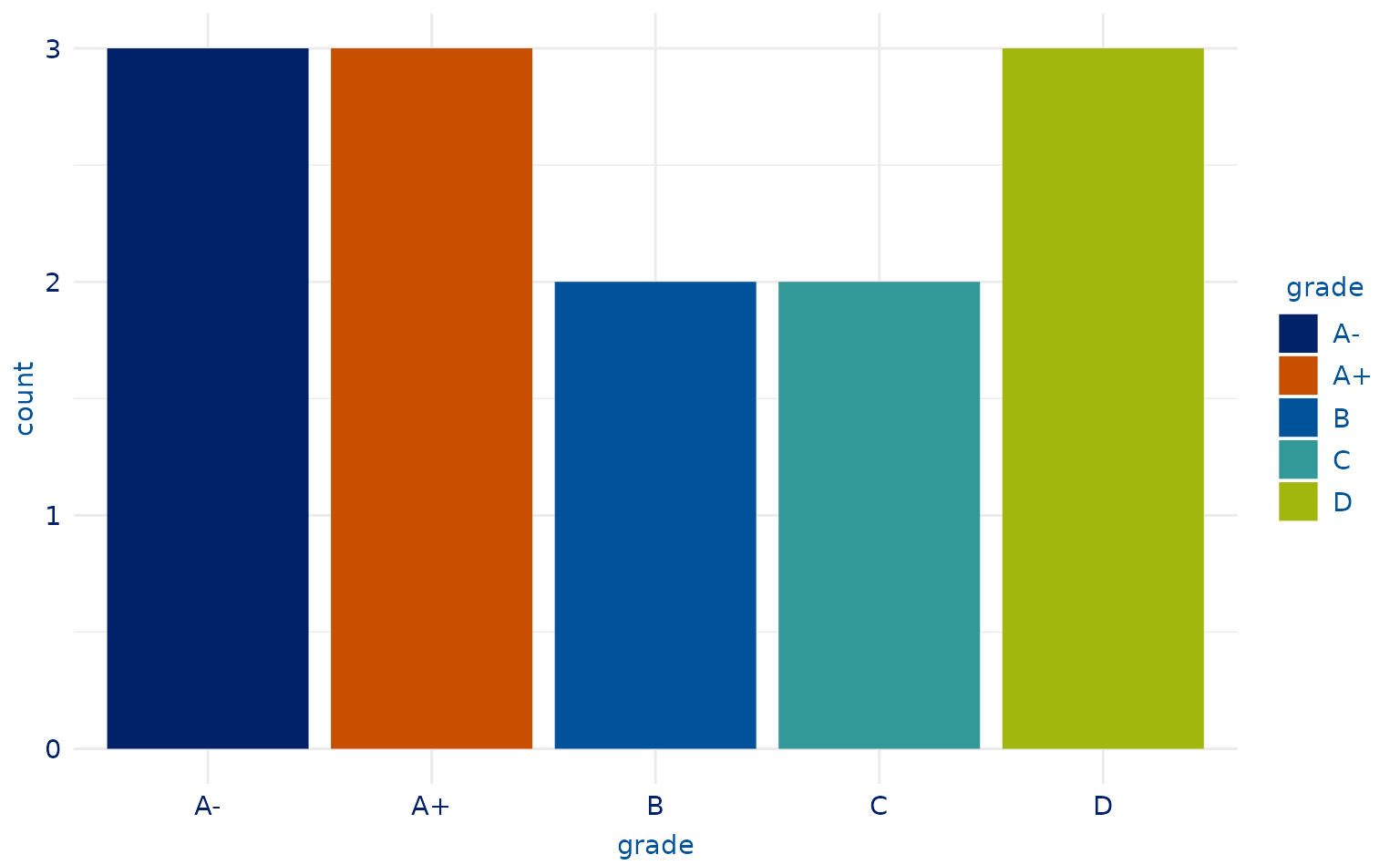
# 4-category plot
plot2.5 <- students %>%
  slice(-c(9, 10, 13, 7, 18, 4, 8)) %>%
  ggplot(aes(x = grade, fill = grade)) +
  geom_bar()

plot2.5 +
  scale_duke_fill_discrete() +
  theme_duke()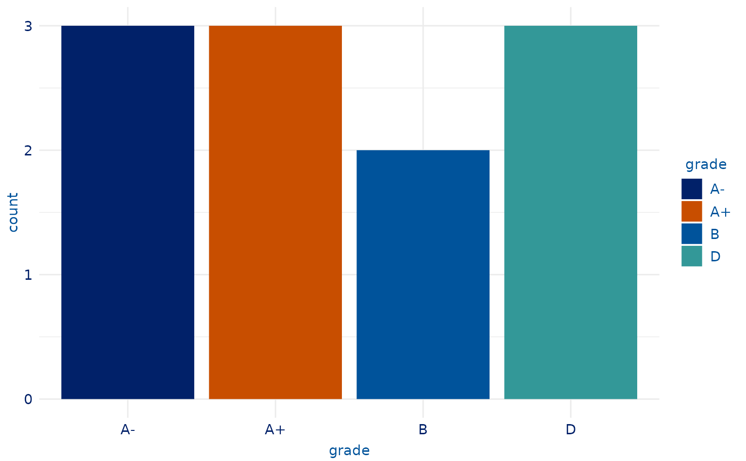
Histogram
plot3 <- ggplot2::ggplot(penguins, aes(body_mass_g)) +
  geom_histogram(ggplot2::aes(fill = species), alpha = 0.8) +
  labs(title = "Distribution of Penguin Body Mass", caption = "(Colors used) \n Duke Royal Blue, Duke Navy Blue, Copper", x = "Body Mass (g)", y = "Count")

plot3 +
  scale_duke_fill_discrete() +
  theme_duke()
#> `stat_bin()` using `bins = 30`. Pick better value with `binwidth`.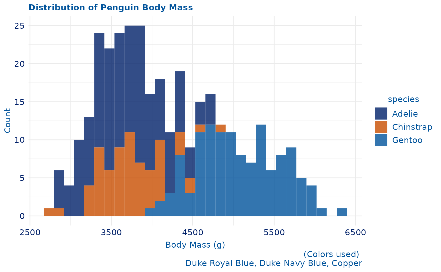
plot3 +
  scale_duke_fill_discrete() +
  theme_minimal()
#> `stat_bin()` using `bins = 30`. Pick better value with `binwidth`.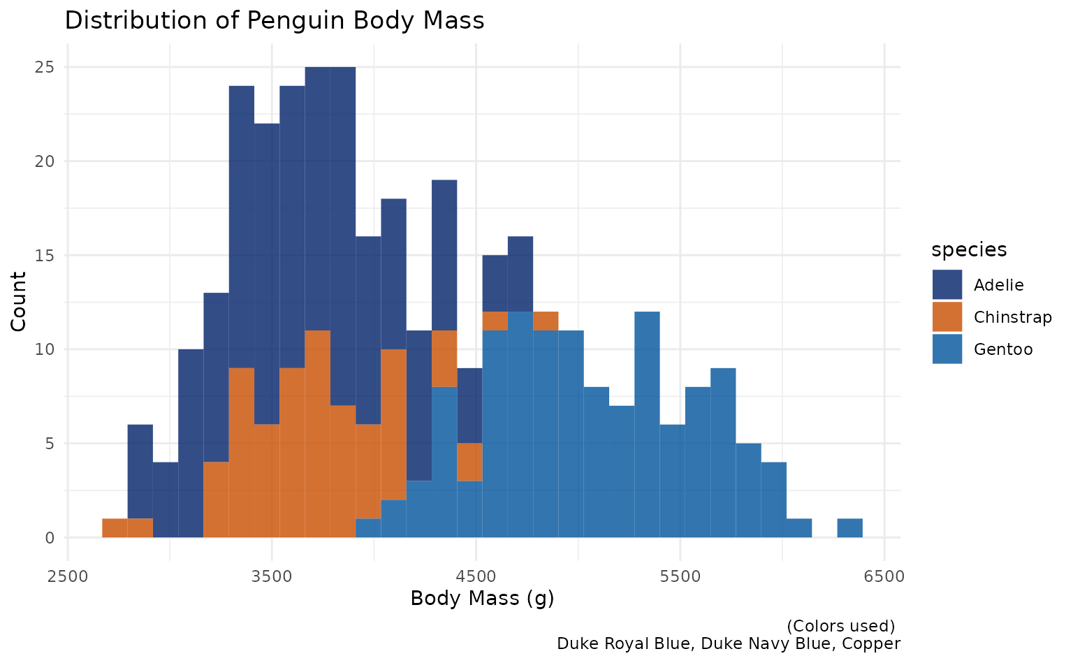
Box Plot
plot4 <- ggplot2::ggplot(penguins, ggplot2::aes(sex, body_mass_g)) +
  ggplot2::geom_boxplot() +
  ggplot2::labs(title = "Comparison of Body Mass By Sex", x = "Sex", y = "Body Mass (g)")

plot4 +
  theme_duke()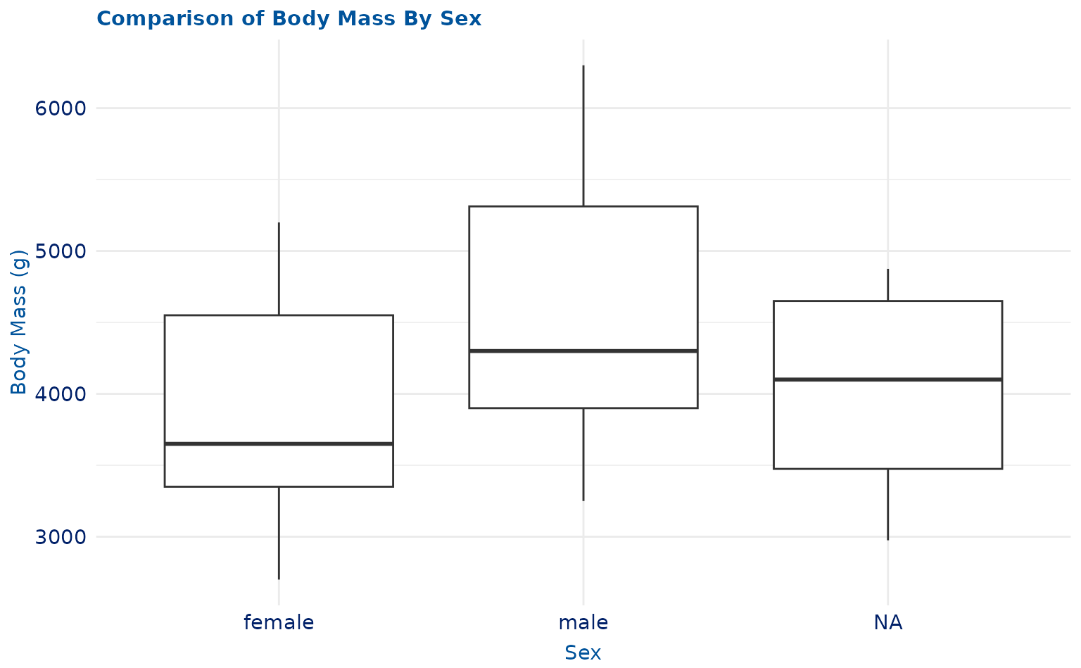
plot4 +
  theme_minimal()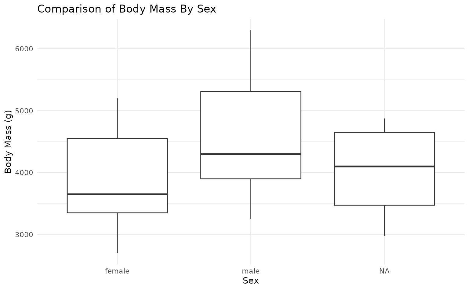
Density Plot
plot5 <- ggplot2::ggplot(penguins, ggplot2::aes(bill_depth_mm)) +
  ggplot2::geom_density(ggplot2::aes(fill = species)) +
  ggplot2::labs(title = "Density of Penguin Bill Depth", x = "Bill Depth (mm)", y = "Densiy")

plot5 +
  scale_duke_fill_discrete() +
  theme_duke()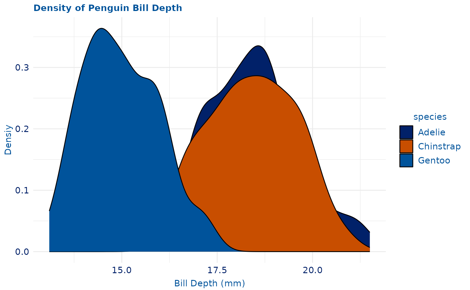
plot5 +
  scale_duke_fill_discrete() +
  theme_minimal()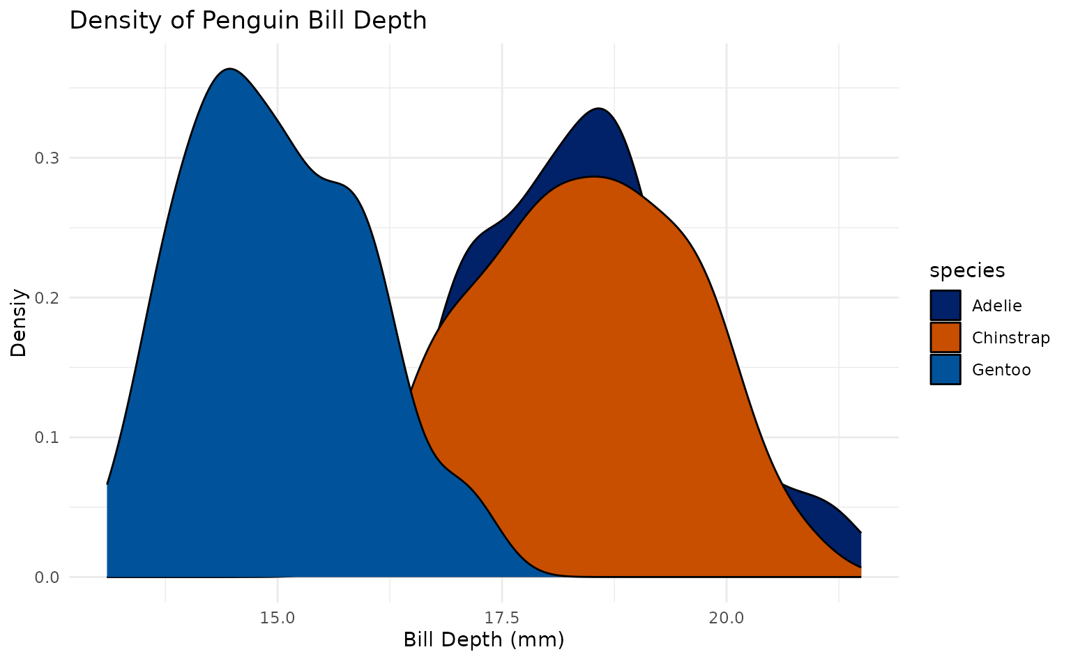
Jitter Plot - Discrete Color
plot6 <- ggplot2::ggplot(penguins, ggplot2::aes(year, body_mass_g)) +
  ggplot2::geom_jitter(ggplot2::aes(color = species)) +
  ggplot2::labs(title = "Comparison of Body Mass By Year", x = "Year", y = "Body Mass (g)")

plot6 +
  scale_duke_color_discrete() +
  theme_duke()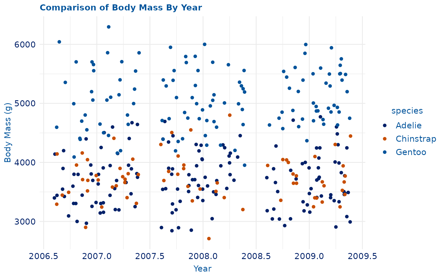
plot6 +
scale_duke_color_discrete() +
theme_minimal()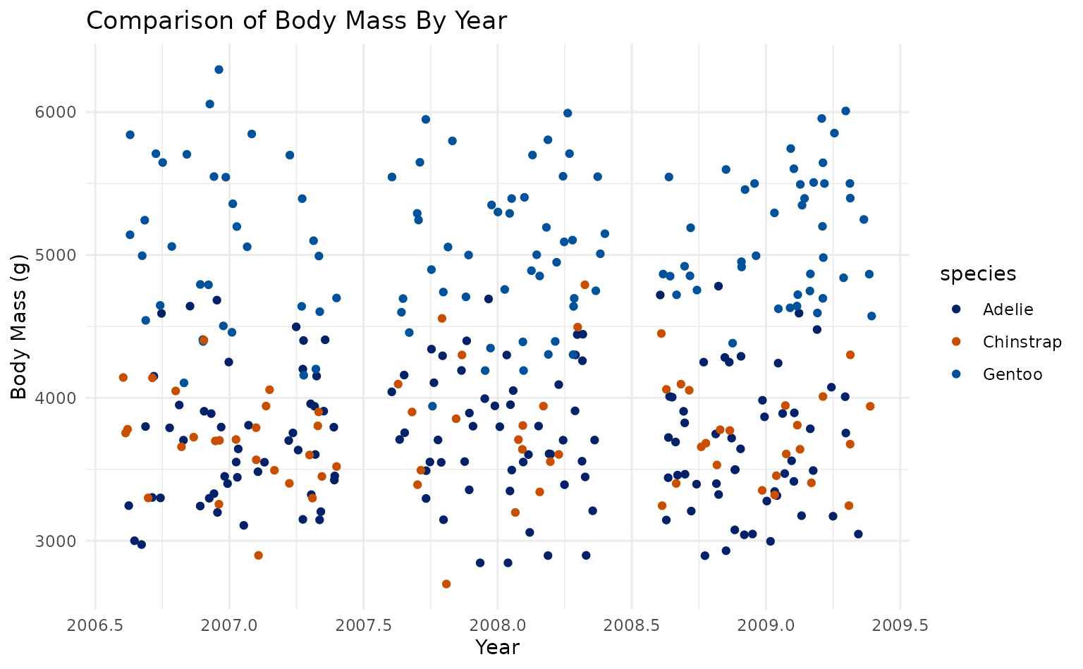 ## Jitter Plot - Discrete Color
plot6.1 <- ggplot2::ggplot(penguins, ggplot2::aes(year, body_mass_g)) +
  ggplot2::geom_jitter(ggplot2::aes(color = bill_length_mm)) +
  ggplot2::labs(title = "Comparison of Body Mass By Year", x = "Year", y = "Body Mass (g)")

plot6.1 +
  scale_duke_continuous() +
  theme_duke()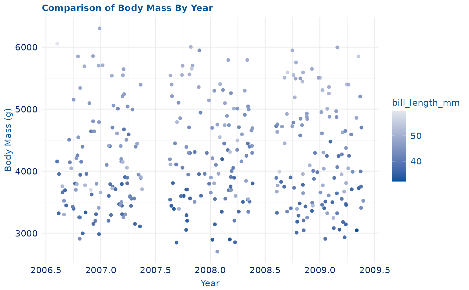
plot6.1 +
  scale_duke_continuous() +
  theme_minimal()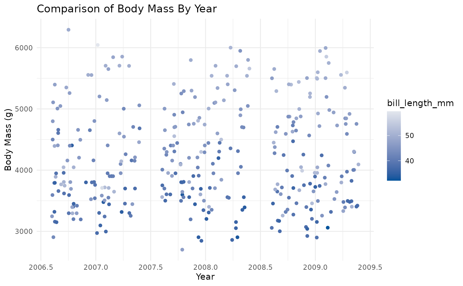
Line Plot
yearly_avg <- penguins %>%
  filter(!is.na(bill_length_mm)) %>%
  group_by(island, year) %>%
  summarize(island, year, mean = mean(bill_length_mm)) %>%
  distinct(island, year, .keep_all = T)
#> `summarise()` has grouped output by 'island', 'year'. You can override using
#> the `.groups` argument.

lineplot <- ggplot(data = yearly_avg, aes(x = as.factor(year), y = mean, group = island)) +
  geom_line(aes(color = island), linewidth = 1) +
  geom_point(aes(color = island)) +
  labs(title = "Average Island Bill Length(mm) Per Year", x = "Year", y = "Average Bill Length (mm)") +
  theme_duke() +
  scale_duke_color_discrete()
lineplot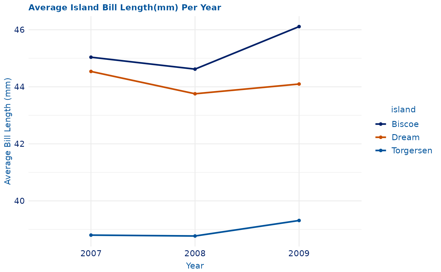
# with point shape and line pattern
lineplot.2 <- ggplot(data = yearly_avg, aes(x = as.factor(year), y = mean, group = island)) +
  geom_line(aes(color = island, linetype = island), linewidth = 1) +
  geom_point(aes(color = island, shape = island)) +
  labs(title = "Average Island Bill Length(mm) Per Year", x = "Year", y = "Average Bill Length (mm)") +
  theme_duke() +
  scale_duke_color_discrete()
lineplot.2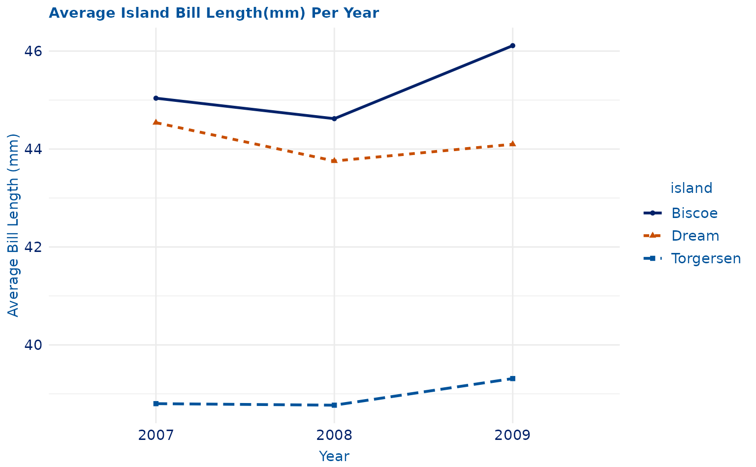
Mosaic Plot
plot7 <- ggplot(data = penguins) +
  ggmosaic::geom_mosaic(aes(x = ggmosaic::product(sex, island), fill = sex)) +
  labs(title = "Penguin Sex vs. Island", x = "Island", y = "Penguin Sex", caption = "(Color from top to bottom) \n Granite, Duke Navy Blue, Duke Royal Blue")

plot7 +
  scale_duke_fill_discrete() +
  theme_duke()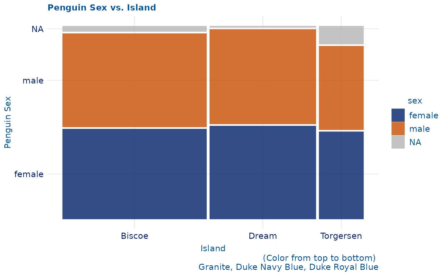
plot7 +
  scale_duke_fill_discrete() +
  theme_minimal()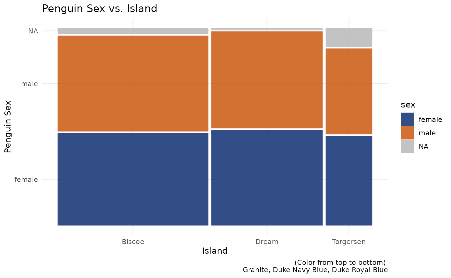
Label Plot
plot8 <- ggplot2::ggplot(penguins, ggplot2::aes(bill_length_mm, bill_depth_mm, fill = island)) +
  ggplot2::geom_label(aes(label = island)) +
  ggplot2::labs(title = "Bill Length/Depth by Island", x = "Bill Length (mm)", y = "Bill Depth (mm)")

plot8 +
  scale_duke_fill_discrete() +
  theme_duke()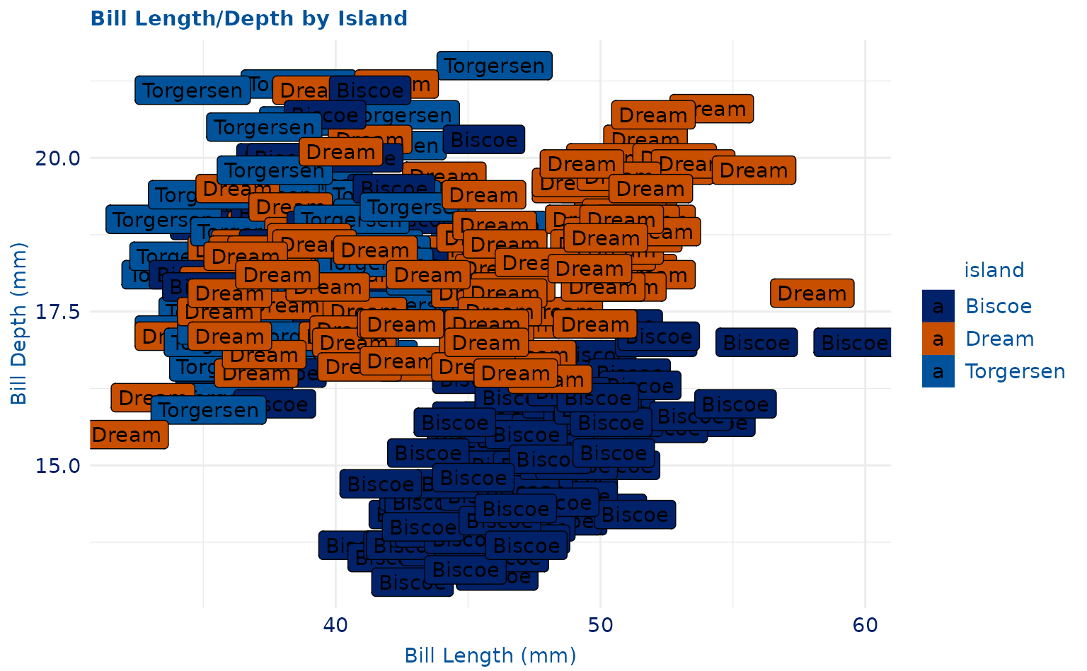
plot8 +
  scale_duke_fill_discrete() +
  theme_minimal()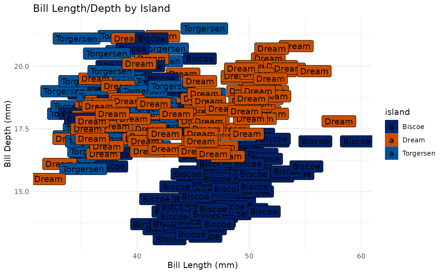
Quantile Plot
plot9 <- ggplot2::ggplot(penguins, ggplot2::aes(bill_length_mm, bill_depth_mm, color = species)) +
  ggplot2::geom_quantile() +
  ggplot2::labs(title = "Bill Length/Depth Quantiles", x = "Bill Length (mm)", y = "Bill Depth (mm)")

plot9 +
  scale_duke_color_discrete() +
  theme_duke()
plot9 +
  scale_duke_color_discrete() +
  theme_minimal()
Area Plot
plot10 <- ggplot2::ggplot(penguins, ggplot2::aes(body_mass_g, fill = species)) +
  ggplot2::geom_area(stat = "bin") +
  ggplot2::labs(title = "Area of Body Mass Index", x = "BMI")

plot10 +
  scale_duke_fill_discrete() +
  theme_duke()
#> `stat_bin()` using `bins = 30`. Pick better value with `binwidth`.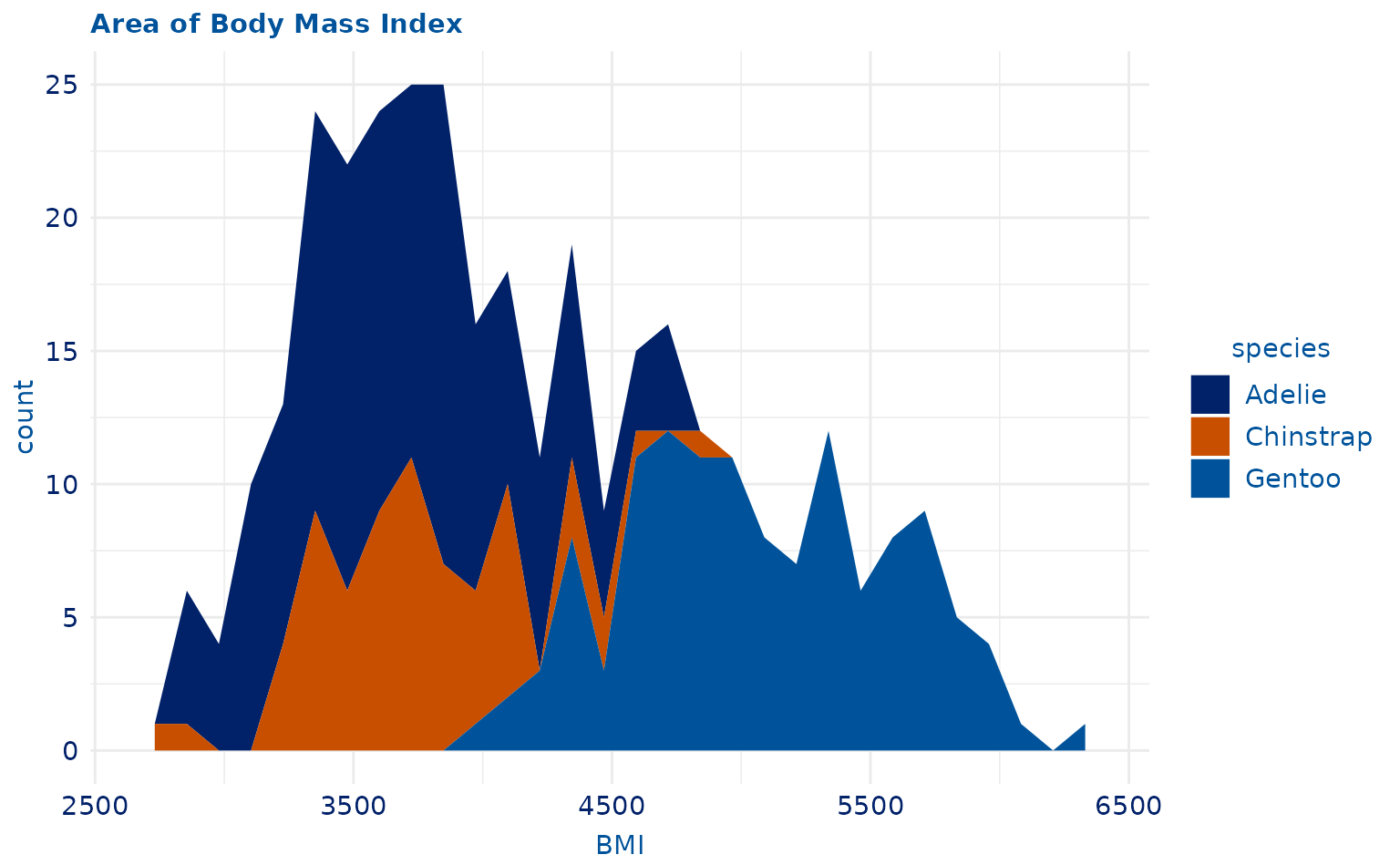
plot10 +
  scale_duke_fill_discrete() +
  theme_minimal()
#> `stat_bin()` using `bins = 30`. Pick better value with `binwidth`.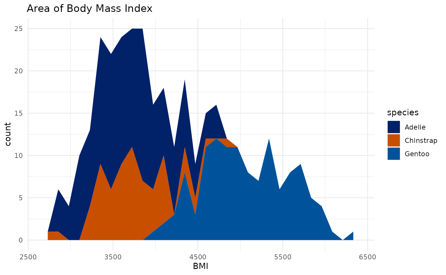
Dot Plot
plot11 <- ggplot2::ggplot(penguins, ggplot2::aes(body_mass_g)) +
  ggplot2::geom_dotplot(aes(fill = species)) +
  ggplot2::labs(title = "Dotplot of BMI", x = "BMI")

plot11 +
  scale_duke_fill_discrete() +
  theme_duke()
#> Bin width defaults to 1/30 of the range of the data. Pick better value with
#> `binwidth`.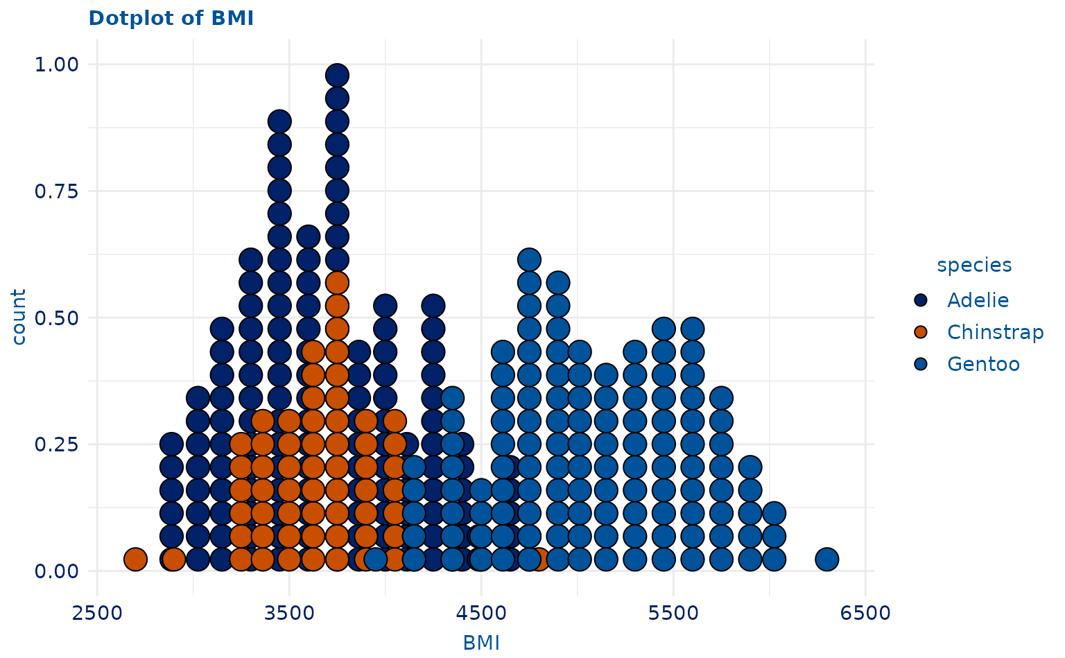
plot11 +
  scale_duke_fill_discrete() +
  theme_minimal()
#> Bin width defaults to 1/30 of the range of the data. Pick better value with
#> `binwidth`.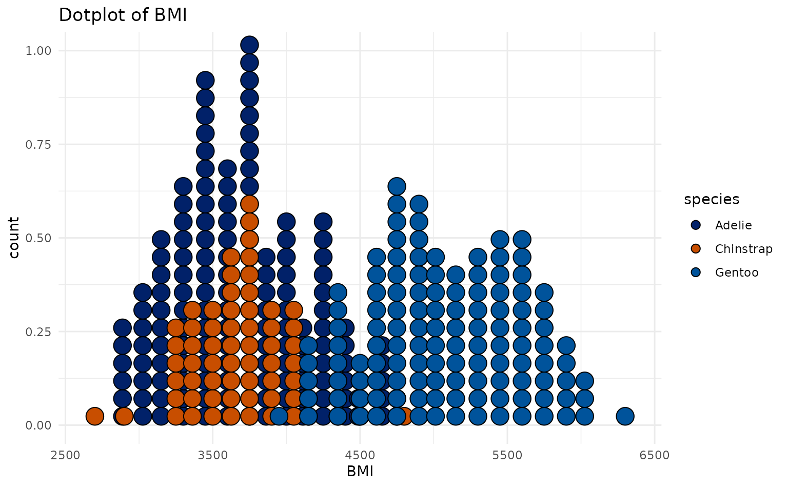
Frequency Polynomial Plot
plot12 <- ggplot2::ggplot(penguins, ggplot2::aes(body_mass_g)) +
  ggplot2::geom_freqpoly(aes(color = species)) +
  ggplot2::labs(title = "Frequency Polynomial Plot of BMI", x = "BMI")

plot12 +
  scale_duke_color_discrete() +
  theme_duke()
#> `stat_bin()` using `bins = 30`. Pick better value with `binwidth`.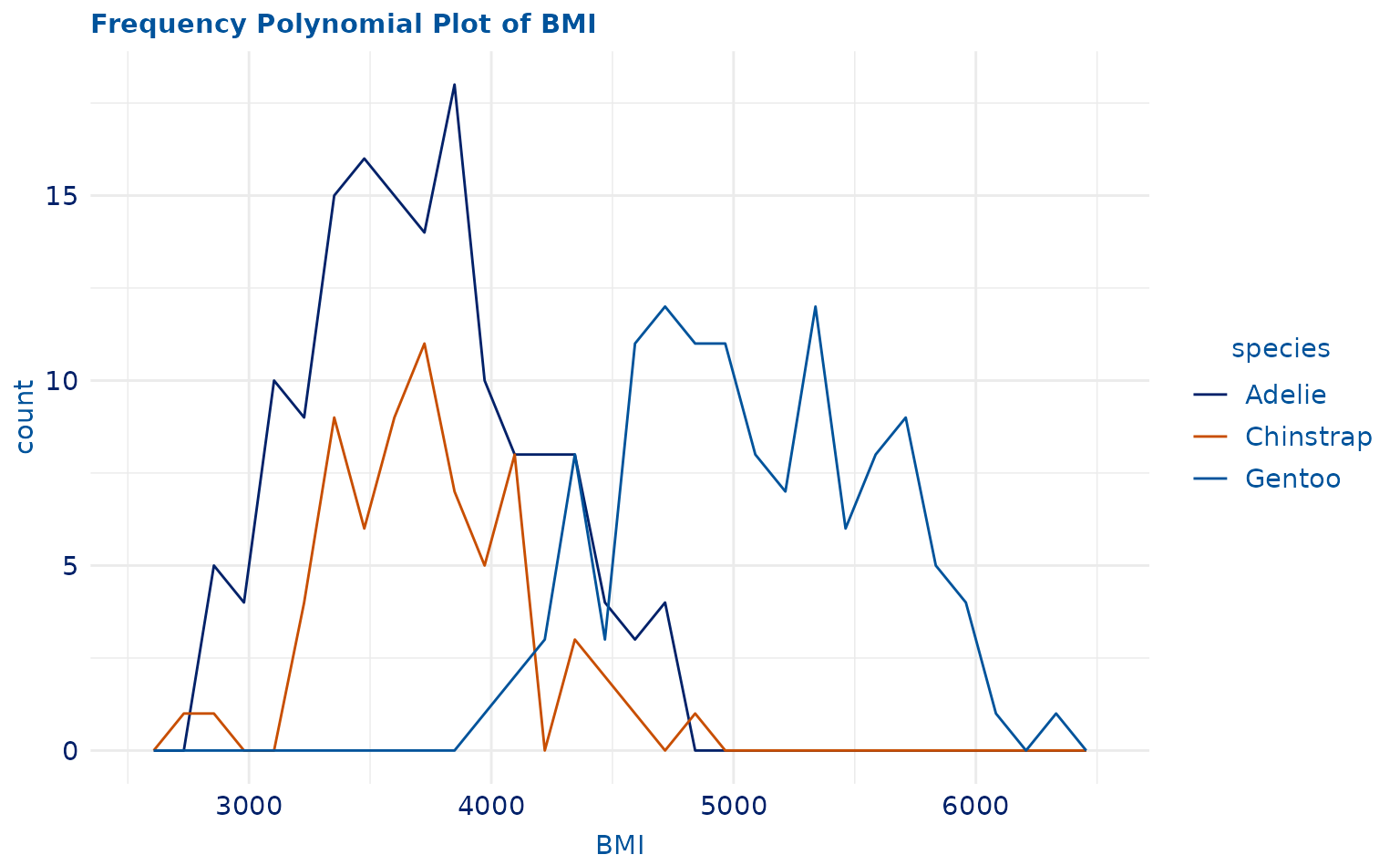
plot12 +
  scale_duke_color_discrete() +
  theme_minimal()
#> `stat_bin()` using `bins = 30`. Pick better value with `binwidth`.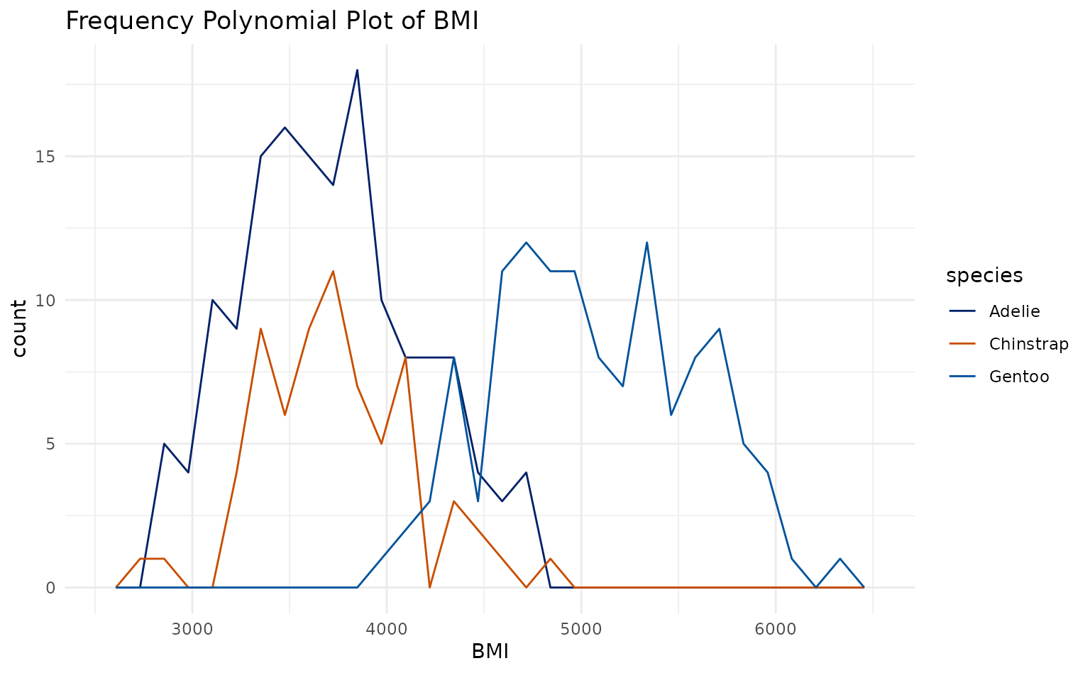
Column Plot
plot13 <- ggplot2::ggplot(penguins, ggplot2::aes(species, body_mass_g, color = species)) +
  ggplot2::geom_col() +
  ggplot2::labs(title = "BMI By Species of BMI", x = "Species", y = "BMI")

plot13 +
  scale_duke_color_discrete() +
  theme_duke()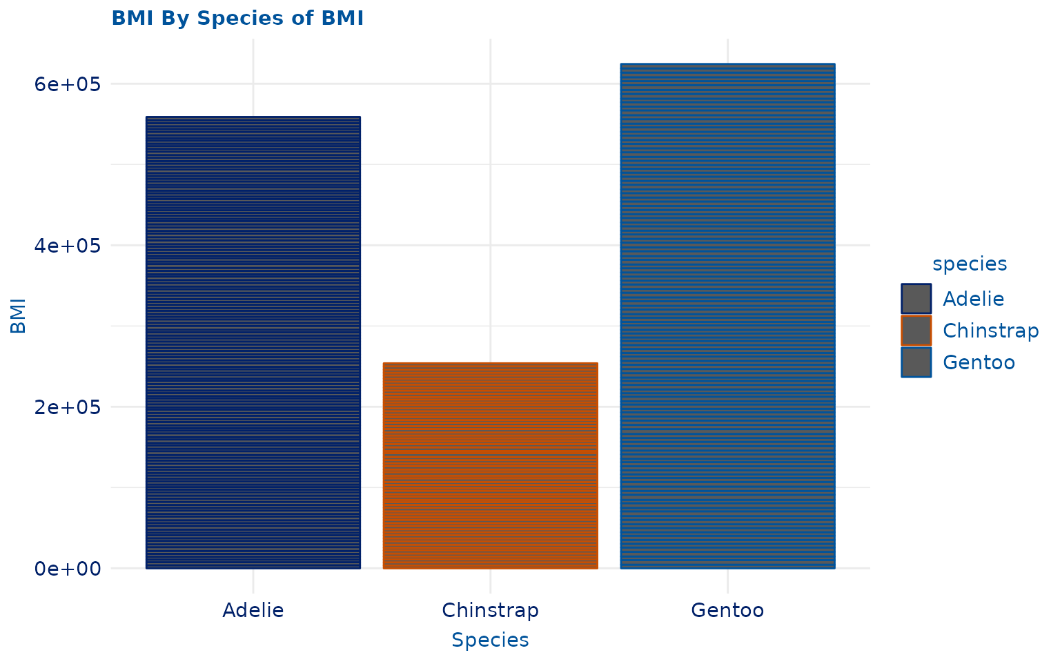
plot13 +
  scale_duke_color_discrete() +
  theme_minimal()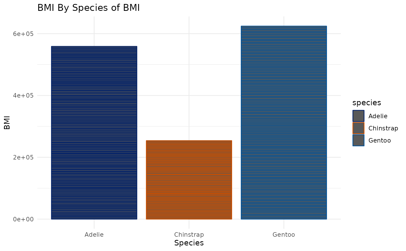
Violin Plot
plot14 <- ggplot2::ggplot(penguins, ggplot2::aes(species, body_mass_g, fill = species)) +
  geom_violin(scale = "area") +
  ggplot2::labs(title = "BMI By Species", x = "Species", y = "BMI")

plot14 +
  scale_duke_fill_discrete() +
  theme_duke()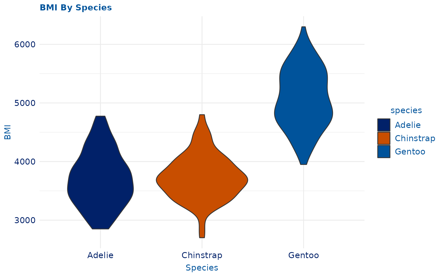
plot14 +
  scale_duke_fill_discrete() +
  theme_minimal()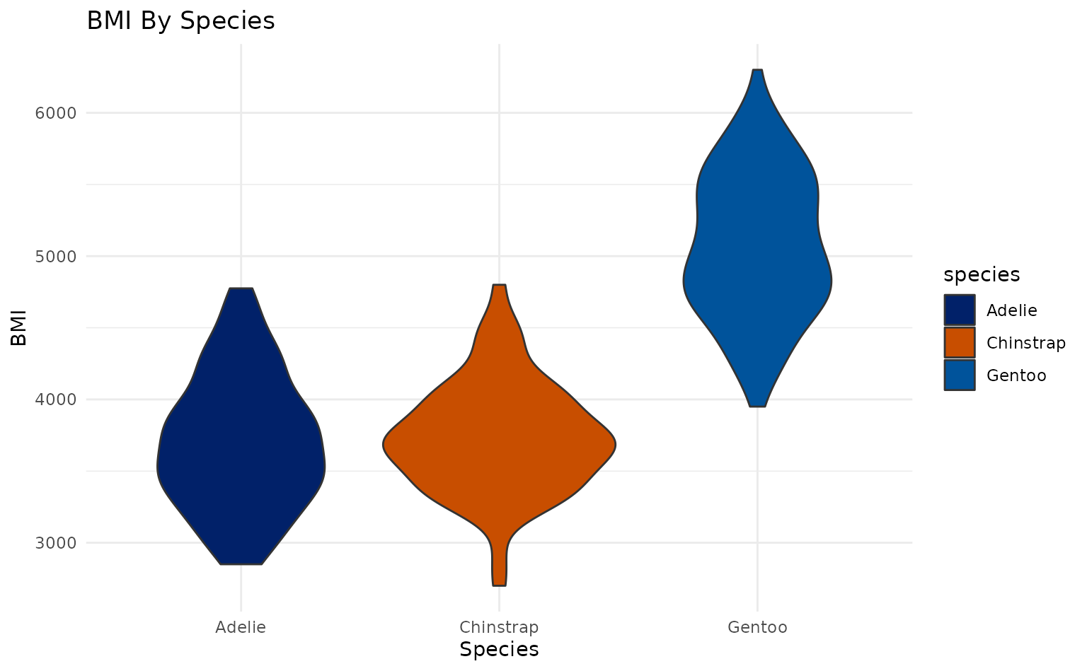
Count Plot
plot15 <- ggplot2::ggplot(penguins, ggplot2::aes(species, island, color = species)) +
  geom_count() +
  ggplot2::labs(title = "Species Count by Island", x = "Species", y = "Island")

plot15 +
  scale_duke_color_discrete() +
  theme_duke()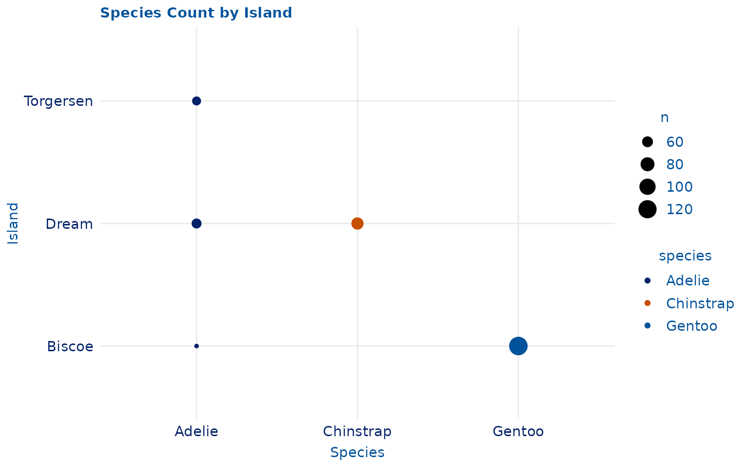
plot15 +
  scale_duke_color_discrete() +
  theme_minimal()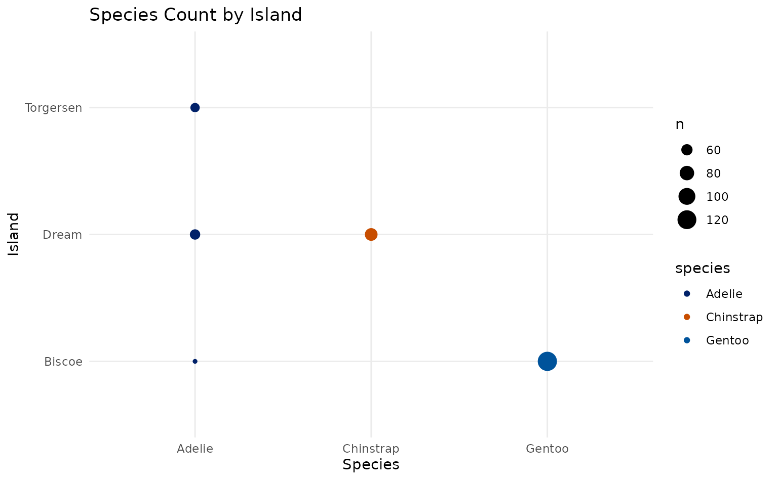
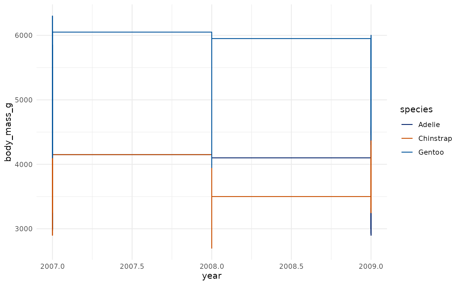
Step Plot
plot16 <- ggplot2::ggplot(penguins, ggplot2::aes(year, body_mass_g, color = species)) +
  geom_step()
ggplot2::labs(title = "BMI By Year", x = "Year", y = "BMI")
#> $x
#> [1] "Year"
#>
#> $y
#> [1] "BMI"
#>
#> $title
#> [1] "BMI By Year"
#>
#> attr(,"class")
#> [1] "labels"

plot16 +
  scale_duke_color_discrete() +
  theme_duke()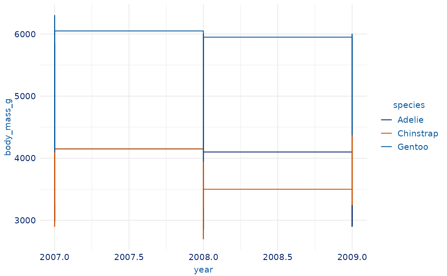
plot16 +
  scale_duke_color_discrete() +
  theme_minimal()